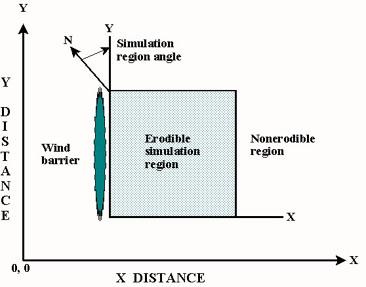
Figure 1. Schematic of simulation region
Introduction
The objective of the erosion submodel is to simulate the components of soil loss/deposition over a rectangular field in response to wind speed , wind direction, field orientation, and surface conditions on a sub-hourly basis (Fig. 1). In WEPS barriers maybe placed on any or all field boundaries. When barriers are present, the wind speed is reduced in the sheltered area on both the upwind and downwind sides of the barriers. The submodel determines the threshold friction velocity at which erosion can begin for each surface condition. When wind speeds exceed the threshold, the submodel calculates the loss/deposition over a series of individual grid cells representing the field. The soil/loss deposition is divided into components of saltation/creep and suspension, because each has different transport modes, as well as off-site impacts. Finally, the field surface is periodically updated to simulate the changes caused by erosion. The purpose of this paper is to provide users with a brief overview of the submodel. For an in-depth description of the equations used in this submodel, see the WEPS Erosion Submodel Technical Description (Hagen, 1995).
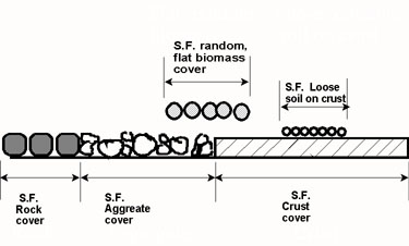
Figure 2. Diagram illustrating compoments of flat surface vover inputs to the Erosion submodel.
Surface Conditions Needed as Submodel Inputs
Surface roughness is represented by both random roughness and oriented roughness. The parameters used are standard deviation of the surface heights for
random roughness and the height and spacing of ridges for oriented roughness.
Surface cover is represented on three levels (Fig. 2). In the first level, surface rock, aggregates and crust comprise 100 percent of the cover. In the second level, the parameter is the fraction of the crusted surface covered with loose, erodible soil. When there is no crust, this parameter is always zero. In the third level, the parameter is the fraction of total surface covered by flat, random biomass.
The aggregate density and size distribution are input parameters that indicate soil mobility. The dry mechanical stability of the clods/crust are input parameters
that indicate their resistance to abrasion from impacts by eroding soil. Surface soil wetness is also input and used to increase the threshold friction velocity at
which erosion begins.
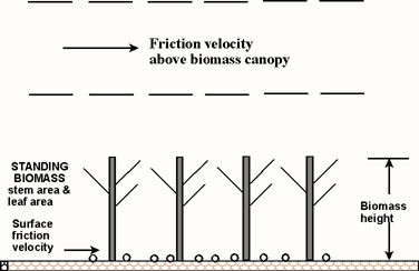
Figure 3. Diagram illustrating friction velocity above standing biomass that is reduced by drag of stems and leaves to the surface friction velocity below the standing biomass.
Uniformly distributed, standing biomass is 5 to 10 times more effective in controlling wind erosion than flat biomass, and thus, is treated separately. The wind
friction velocity above standing biomass is depleted by the leaves and stems to obtain the surface friction velocity at the surface that is used to drive erosion
(Fig. 3). Leaves are represented by a leaf area index and stems by a stem silhouette area index in the input parameters.
Erosion Processes Simulated in the Submodel
Soil transport during wind erosion occurs in three modes: creep-size aggregates, 0.84-2.0 mm (0.033 - 0.079 in.) in diameter roll along the surface,
saltation-size aggregates, 0.10 - 0.84 mm (0.004 - 0.033 in.) in diameter hop over the surface, and suspension-size aggregates, < 0.01 mm ( 0.004 in.) in
diameter move above the surface in the turbulent flow. Obviously, variations in friction velocity, aggregate density and sediment load may change the mass of
aggregates moving in a given mode. Saltation and creep are simulated together, because they have a limited transport capacity that depends mainly upon
friction velocity and surface roughness. The suspension component is simulated with no upper limit on its transport capacity at the field scale. A portion of the
suspension component also is simulated as PM-10, i.e., particulate matter less than 10 micrometers (0.0004 in.) in diameter that is regulated as a health hazard.
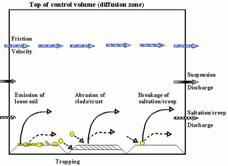
Figure 4. Diagram illustrating processes simulated by the Erosion submodel on a bare soil surface in an indivifual grid cell.
Multiple, physical erosion processes are simulated in the erosion submodel, and these are illustrated for a single grid cell in Fig. 4. The two sources of
eroding soil are emission of loose soil and entrainment of soil abraded from clods and crust. These sources are apportioned between saltation/creep and
suspension components based on the process and soil characteristics. Three processes deplete the amount of moving saltation/creep. These include trapping in
surface depressions, interception by plant stems/leaves, and breakage of saltation/creep to suspension-size.
Simulation of surface rearrangement is accomplished by allowing emissions to deplete the loose soil and armor the surface in the upwind field area. In contrast,
processes such as abrasion of the protruding aggregates and trapping in depressions dominate in downwind areas and lead to smoothing the surface and a
build-up of loose saltation/creep. A build-up of saltation/creep often occurs, because the transport capacity may be satisfied, but abrasion of clods/crust
continues to create additional saltation/creep-size soil.
![]()
Figure 5. Diagram illustrating downwind transport capacity for saltation & creep, but a continuing increase in transported mass of suspension-size soil downwind.
Typical behavior of the downwind soil discharge simulated along a line transect for the saltation/creep and suspension components is illustrated in Fig. 5. The suspension component keeps increasing with downwind distance even though saltation/creep reaches transport capacity. This is because the sources for suspension-size soil are usually active over the entire field. These sources include emissions from impacts on loose soil, abrasion from clods/crust, and breakage from impacting saltation/creep-size aggregates. Moreover, the suspension component has a transport capacity many times larger than that of saltation/creep, so on large fields it is the 'freightliner' for moving soil and saltation/creep is merely the 'pickup truck'.
Outputs From the Erosion Submodel
The Erosion submodel calculates total, suspension, and PM-10 soil loss/deposition at each grid cell in the field. The grid cell data are summarized in other
parts of WEPS and reported to users as averages over the field for selected periods. The submodel also calculates the components of soil discharge crossing
each field boundary. These are reported to users based on the size ranges of aggregates as saltation/creep, suspension, and PM-10. These latter outputs are
useful for evaluating off-site impacts in any given direction from the eroding field.
References
Hagen, L.J. 1995. Wind Erosion Prediction System (WEPS) Technical Description: Erosion submodel. IN Proc. of the WEPP/WEPS Symposium. Soil and Water Conserv. Soc., Des Moines, IA.