Introduction
All the soil properties that control soil wind erodibility vary with time. Hence, the objective of the soil submodel is to simulate these temporal soil properties
on a daily basis in response to various driving processes. On days when wind erosion or management activities occur, the Erosion and Management submodels
may also update some of the same temporal variables. The driving processes that change soil temporal properties are mostly weather related, and hence, the
sequence of occurrence of individual driving processes is highly variable. Thus, the submodel must be able to update the soil variables given an arbitrary
driving process and the soil conditions for the prior day. The purpose of this paper is to provide a brief overview of the major processes that are simulated, and
the temporal variables that are updated by the soil submodel. For an in-depth discussion of the equations used in the Soil submodel, see the Soil Submodel
Technical Document (Hagen et al., 1995).
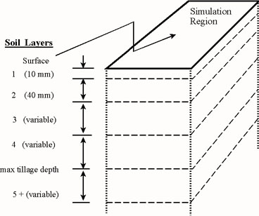
Figure 1. Diagram representing the spatial domain of the Soil submodel.
Spatial Regime for the Submodel
In the Soil submodel, the spatial regime is considered to be uniform in the horizontal direction over the simulation region, but non-uniform in the vertical
direction (Fig. 1). Hence, the vertical direction is divided into layers in each soil profile. Some of the layer boundaries are selected to coincide with the layers
determined by the NRCS Soil Survey of each soil. Layers one and two are initially set at 10 and 40 mm (0.39 and 1.57 inches), respectively, to allow
simulation of sharp gradients in temporal soil properties near the surface.
Soil Layering Scheme
The hydrology and crop sub-models of WEPS depend upon the soil being stratified by layers. Hydrology moves water up and down within the soil based upon the relative wetness of adjacent layers. Crop estimates plant growth based upon several factors, one of the most important being availability of water within the the root zone. It is important that WEPS keep track of now how much water is available at various soil depths. Hence, WEPS views the soil as a series of layers, each layer possibly having distinct physical characteristics but this is not necessary.
WEPS divides the soil into layers based upon National Soil Information System (NASIS) input data. The layering scheme respects the underlying NASIS data. That is, no NASIS layers are combined when creating WEPS layers. Much of the complexity of the layering process is due to the creation of the very thin top layers. The design criteria are:
1. Preserve NASIS layering, i.e. a WEPS layer cannot cross a NASIS layer boundary.
2. Try to get the first three layers to be 10, 40 and 50 mm.
3. Preserve the relative sizes, 1:4:5:5, of the top layers if the absolute size cannot be attained.
4. Divide the remaining layers into relatively uniform thicknesses, somewhat thinner at the top and thicker as depth increases.
Processes Simulated and Variables Updated by the Submodel
The processes simulated and the variables updated are summarized in Table 1. The effect of the processes on roughness is always to reduce the roughness. In contrast, many of the other variables either increase or decrease in value depending upon the prior-day value, soil intrinsic properties and the driving process. To simulate the dry stability and aggregate size distribution, for a wide range of soils, these variables were first normalized using mean and standard deviation of the variables for each soil series to give a range from 0 to 1 for each variable. The driving processes were then applied to the normalized ranges to determine the change in the normalized variable. Finally, the updated normalized values were converted to the real values of these variables.Table 1. Soil submodel variable and process matrix.
| Surface Processes | Layer Processes | |||||
| Soil Temporal Variables | Rain | Sprinkler Irrigate |
Snow Melt | Wet/ dry |
Freeze/ thaw |
Freeze/ dry |
| Roughness: | ||||||
| Ridge Height | X | X | X | |||
| Dike Height | X | X | X | |||
| Random | X | X | X | |||
| Crust: | ||||||
| Depth | X | X | X | |||
| Cover fraction | X | X | X | |||
| Density | X | X | X | |||
| Stability | X | X | X | X | X | X |
| Loose mass | X | X | X | |||
| Loose cover | X | X | X | |||
| Aggregates: | ||||||
| Size distribution | X | X | X | X | X | X |
| Dry stability | X | X | X | X | X | X |
| Density | X | X | X | X | X | X |
| Layers: | ||||||
| Bulk density | X | X | X | |||
In summary, the Soil submodel outputs updated values on a daily basis for each of the variable listed in Table 1 in response to the occurrence of the various
driving processes.
References
Hagen, L.J., T.M. Zobeck, E.L. Skidmore, and I. Elminyawi. 1995b. WEPS technical documentation: soil submodel. SWCS WEPP/WEPS Symposium. Ankeny, IA